
Microsoft Excel offers much more than basic spreadsheet functions. One of its most powerful and widely used features is the VLOOKUP function, which allows users to perform advanced searches within datasets.
Although this function may initially seem complex, especially when entering the correct parameters, it is easier to use than it appears. Below, we’ll guide you through the steps to effectively apply the VLOOKUP formula in Excel.
How to Use VLOOKUP in Excel
Also known as “Vertical Lookup,” the VLOOKUP function in Excel allows users to search for specific data within a column, making it especially useful for large datasets. This function helps retrieve corresponding values from other columns within the selected range.
Understanding the VLOOKUP Formula
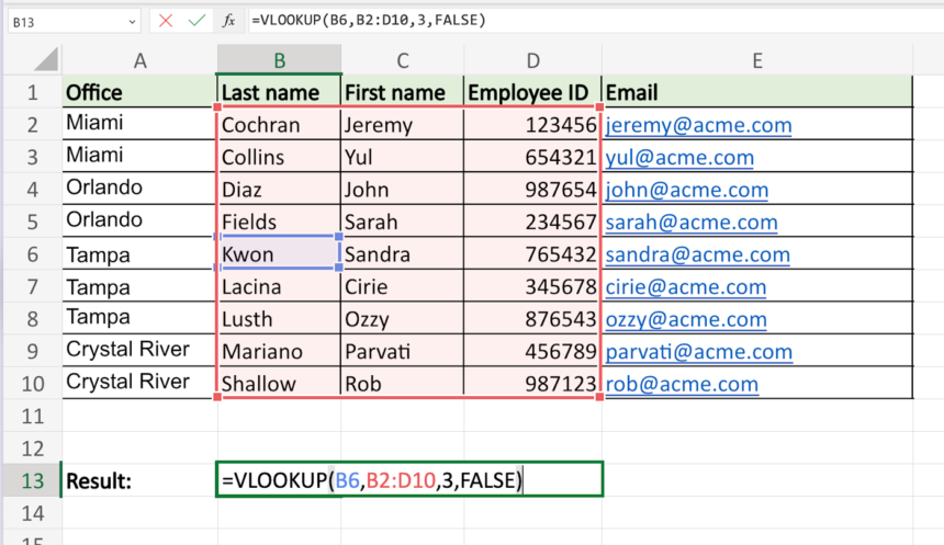
The VLOOKUP formula follows this structure:
=VLOOKUP(lookup_value, table_array, column_index, [range_lookup])
Breaking Down the Formula:
- lookup_value – The value you want to search for.
- table_array – The range of columns where the search will be conducted.
- column_index – The column number (within the selected range) from which the function will return a value.
- range_lookup – Defines whether the search should return an exact match (0 or FALSE) or an approximate match (1 or TRUE).
Step-by-Step Guide to Using VLOOKUP
Follow these steps to apply the VLOOKUP function in Excel:
- Select the cell where you want to insert the formula.
- Enter the search value – In this example, we are searching for a value found in cell G3, so we start with:
=VLOOKUP(G3, - Define the search range – Select the first column of the table where the search will take place.
- Expand the selection – Hold Shift and select the last column in the range. If searching within columns B to D, the formula updates to:
=VLOOKUP(G3, B:D, - Enter the column index – Identify the column containing the value you want to retrieve. If the needed data is in the third column within the selected range, the formula becomes:
=VLOOKUP(G3, B:D, 3, - Specify the search type – Use 0 for an exact match or 1 for an approximate match. For an exact match, the final formula is:
=VLOOKUP(G3, B:D, 3, 0)
Example Usage
If searching for the code “X10003”, the VLOOKUP formula will return “MG” from the corresponding column.
By following these steps, you can efficiently use VLOOKUP to locate and retrieve data in Excel easily.
What is the VLOOKUP formula in Excel for?
Beyond simply searching for items, VLOOKUP is also essential for linking data between tables. This function helps eliminate duplicates, reduce manual errors, and maintain data consistency by retrieving information from one table and displaying it in another.
This makes VLOOKUP particularly useful for professionals working with large datasets, where accuracy and organization are crucial-especially when handling extensive spreadsheets.


